Sparse inverse covariance estimation with the graphical lasso
Friedman, J., Hastie, T., Tibshirani, R.
Keith Hughitt
Graphical Models
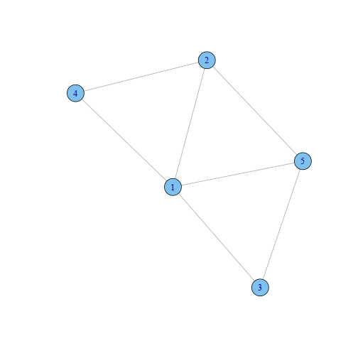
Graphical models provide a way to represent the conditional dependencies between a number of random variables. They provide a visual way of representing the joint distribution of the entire set of RVs.
Components:
- Vertices: random variables
- Edges: condition dependencies between RVs
Types:
- Directed:
Bayesian networks(causal relationships) - Undirected:
Markov random fields/Markov networks
See The Elements of Statistical Learning (ESM) chapter 17 for an overview of undirected graphical models.
Graphical Models
Constructing graphical models from data:
- Model selection: choosing the structure of the graph.
- Learning: Estimating edge weights from data.
ESL p626
Undirected Graphical Models
Gaussian Graphical Models
Assume that the observations have a multivariate Gaussian distribution with mean \(\mu\) and covariance matrix \(\Sigma\).
The inverse covariance matrix \(\Theta = \Sigma^{-1}\) (aka concentration matrix or precision matrix) contains information about the partial covariances between each pair of nodes conditioned on all other variables (ESL.)
If the $ij$th component of \(\Theta\) is zero, then variables \(i\) and \(j\) are conditionally independent, given the other variables.
This is not necessarily true, however, if data is not MV gaussian! (see talk linked to at end of presentation.)
Covariance graphs
- In covariance graphs or relevance networks, edges are present when the covariance is non-zero.
Sparse Graphical Models
- In some cases, you expect that the underlying data should be sparse.
- Want to only keep significant edges.
- An \(L_1\) penalty on the estimation of \(\Sigma^{-1}\) can be used to induce sparseness.
Cell Signaling
Cell signaling
The basic goal of cell signaling to provide a mechanism for cells to respond convey a message from one part of a cell to another.
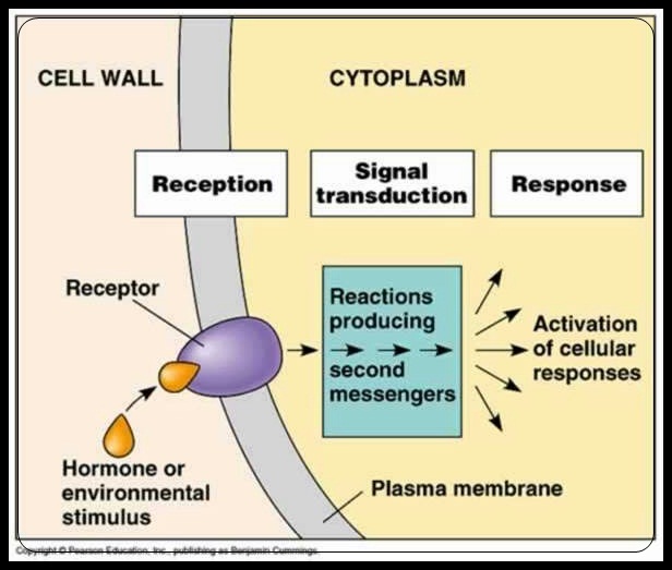
http://commons.wikimedia.org/wiki/File:1Signal_Transduction_Pathways_Model.jpg
Cell signaling
Examples of cell signaling
- Cell to cell communication (e.g. quorum sensing)
- Responding to host (or pathogen) molecules
- Respond to external physiological, nutrient, etc. conditions
- Chemotaxis (movement)
Cell signaling
Cell membrane
Cell signaling often begins at the cell membrane ("Signal transduction").
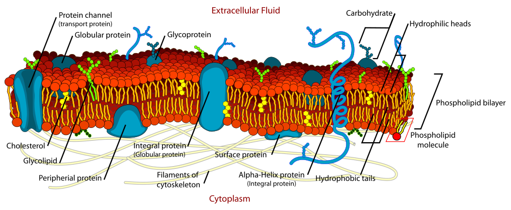
Source: http://en.wikipedia.org/wiki/File:Cell_membrane_detailed_diagram_en.svg
Cell signaling
Lipid rafts
Lipid rafts help to bring together components that function together for a particular signaling pathway: receptors, co-receptors, etc.
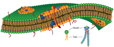
source: http://www.lanl.gov/science/1663/august2011/story3full.shtml
Cell signalling network
It's not quite a 1:1 process...
Sachs 2003; Figure 2
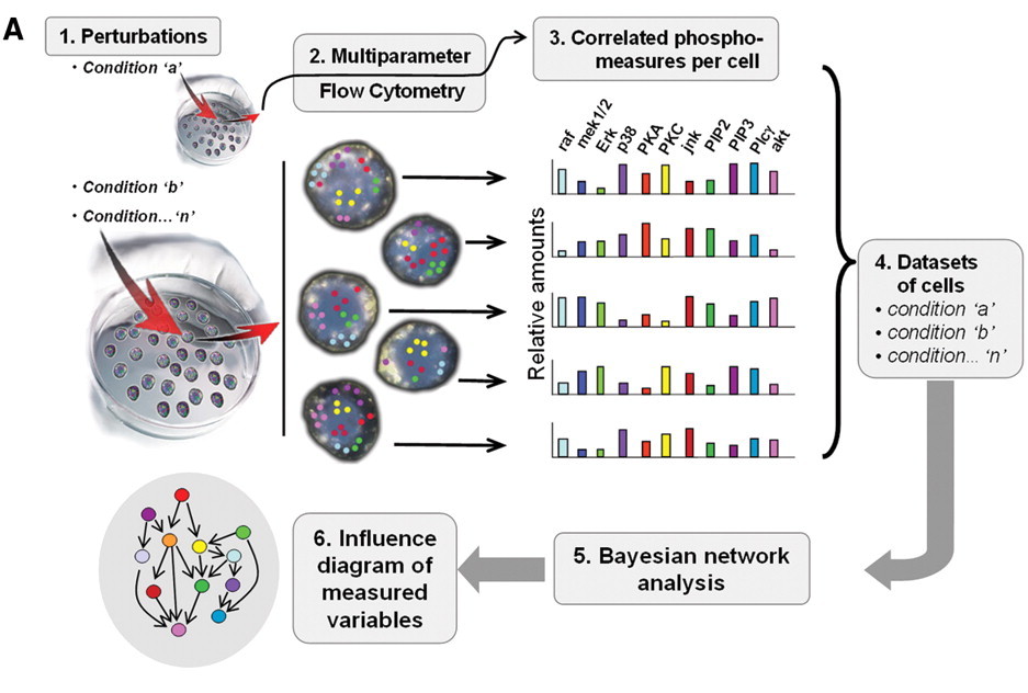
Cell signalling network
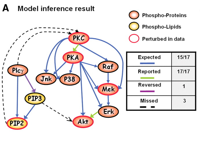
Figure 1A: Network inference using flow cytometry data (Sachs et al 2005)
Flow Cytometry
Flow Cytometry
Flow cytometry a high-throughput single-cell method that is generally used for one of two things:
- Counting cells
- Sorting cells
However, it can also be used to measure many other properties of cells (expression, morphology, enzymatic activity, etc.)
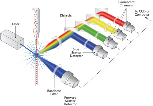
http://www.semrock.com/flow-cytometry.aspx
Flow Cytometry
- Molecules of interest (e.g. proteins involved in a signaling cascade) are "tagged" with an antibody containing a fluorescent protein.
- By using different fluorescent proteins (each of which emits at a different wavelength) multiple proteins can be bound and measured simultaneously.
http://www.antibodies-online.com/resources/17/1247/What+is+flow+cytometry+FACS+analysis/
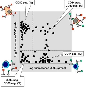
Flow Cytometry
Multicolor Flow Cytometry
- Advantages
- Quantitative
- Can interrogate levels of multiple molecules at the same time
- Processes many individual cells (large \(n\))
- Disadvantages
- Spectral overlap
- Variable brightness of fluorochromes
Flow Cytometry
Spectral Overlap
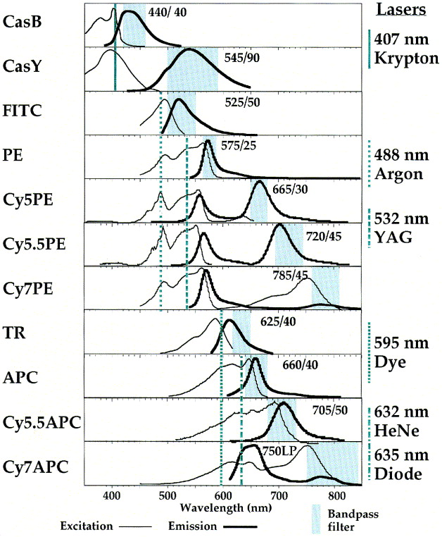
Baumgarth and Roederer, 2000
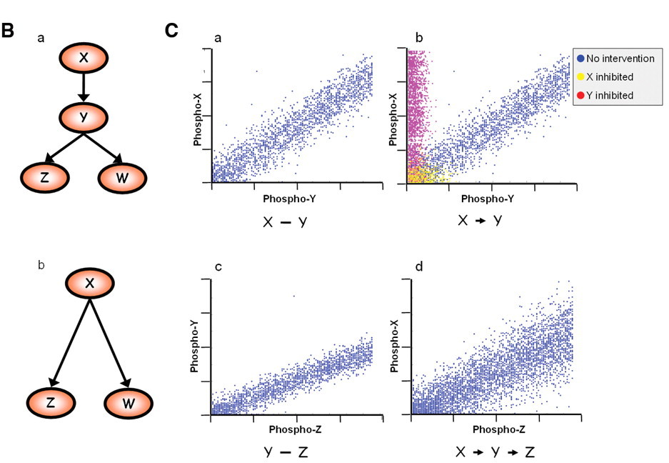
Cell signalling network
Figure 1B-C: Network inference using flow cytometry data (Sachs et al 2005)
Previous Work on Using the Lasso for Sparse Graphical Models
Meinshausen and Bühlmann (2006)
- Which components of \(\Sigma^{-1}\) are non-zero?
- Fit a lasso regression for each variable using all other variables as predictors.
- Considered nonzero if \(\Sigma^{-1}_{ij} \neq 0\) AND/OR \(\Sigma^{-1}_{ji} \neq 0\)
- Shown asymptotically to find nonzero components
Exact solutions
Other authors have suggested exact solutions:
- Yuan & Lin (2007)
- Banerjee et al. (2007)
- Dahl et al. (2007)
Interior point optimization is used to determine an exact maximiation.
Graphical Lasso
- Exact solution based on coordinate descent approach in Banerjee et al. (2007)
Approach
- \(N\) observations, \(x_i, i=1,\ldots,N\) with dimension \(p\), mean \(\mu\) and covariance \(\Sigma\)
- let \(\Theta = \Sigma^{-1}\) and let \(S\) be the empirical covariance matrix: \[S = \frac{1}{N} \sum_{i=1}^N (x_i - \overline{x})(x_i - \overline{x})^T\]
- Goal: Maximize the log-likelihood \[\text{log det} \Theta - \text{tr}(S\Theta) - \rho\Vert \Theta \Vert_1\] over non-negative definite matrices \(\Theta\).
- Above expression is the "Gaussian log-likelihood of the data, partially maximized with respect to the mean parameter \(\mu\).
An interesting methods discussion...
Algorithm (Friedman et al. 2007):
- Start with \(W = S + \rho I\). The diagonal of \(W\) remains unchanged in what follows.
- For each \(j = 1,2,\ldots p,1,2,\ldots p,\ldots,\) solve the lasso problem: \[ min_\beta \{ \frac{1}{2} \Vert W^{1/2}_{11} \beta - b\Vert^2 + \rho \Vert \beta \Vert_1 \}\] where \(b = W^{-1/2}_{11} s_{12}\), which takes as input the inner products \(W_{11}\) and \(s_{12}\). This gives a \(p -1\) vector solution \(\hat{\beta}\). Fill in the corresponding row and column \(W\) using \(w_{12} = W_{11} \hat{\beta}\).
- Continue to convergence.
In glasso, the procedure stops when the average absolute change in \(W\) is
less than \(t \cdot \text{ave} |S^{-\text{diag}}|\) where \(S^{-\text{diag}}\) are
the off-diagonal elements of the empirical coveriance matrix \(S\) and \(t\) is
a fixed threshold, set by default at 0.001.
An interesting algorithm discussion...
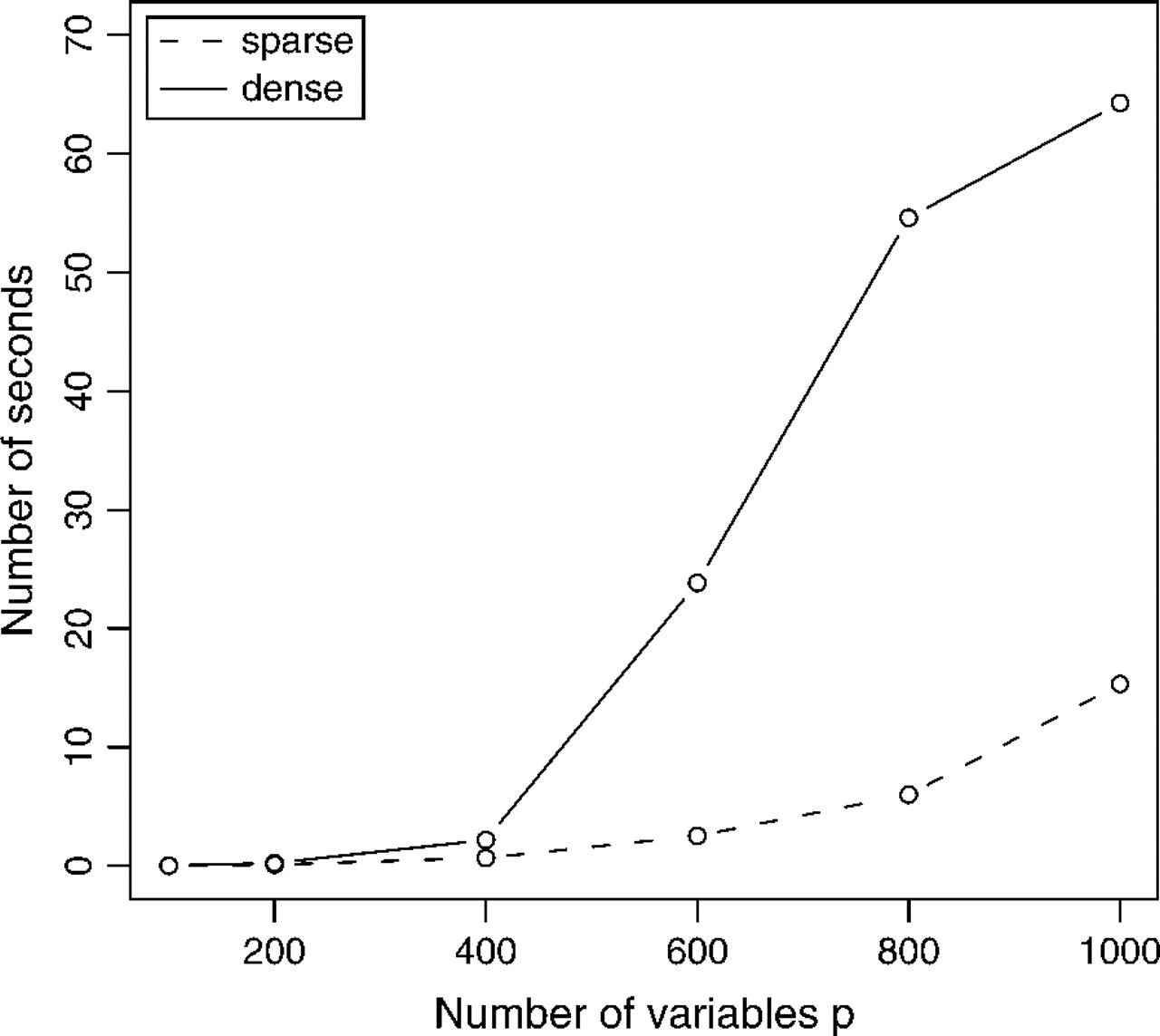
Performance of Graphical Lasso
Performance
- Simulated data for sparse and dense scenarios:
Sparse
- \((\Sigma^{-1})_{ii} = 1\),
- \((\Sigma^{-1})_{i,i-1} = (\Sigma^{-1})_{i-1,i} = 0.5\)
- 0 otherwise
Dense
- \((\Sigma^{-1})_{ii} = 2\),
- \((\Sigma^{-1})_{ii'} = 1\) otherwise
Compared performance to
COVSELmethod from Banerjee et al. (2007).Result: Graphical lasso is 30-4000 times faster than COVSEL and 2-10 slower than the approximate method.
Even for dense problems, finishes in ~1min for p=1000 features. (Hard to tell from graph how it will scale to many more features, however).
Performance
How does the graphical lasso perform on real-world data?
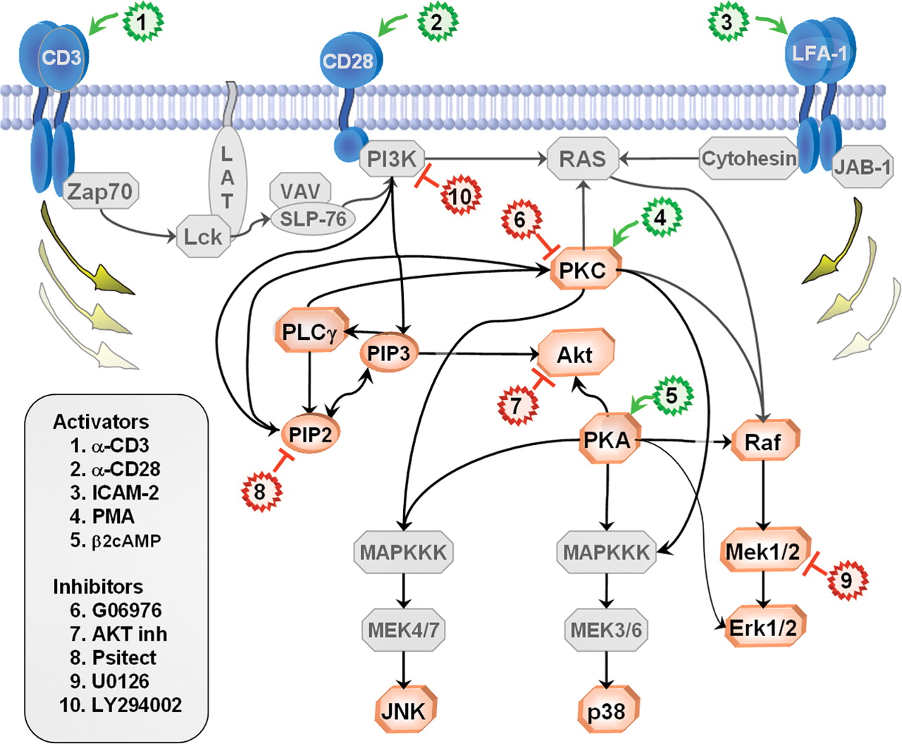
Cell signalling network
To demonstrate the usefulness of the graphical lasso on real-world problems, the method is applied to cytometry data from Sachs et al. (2003)
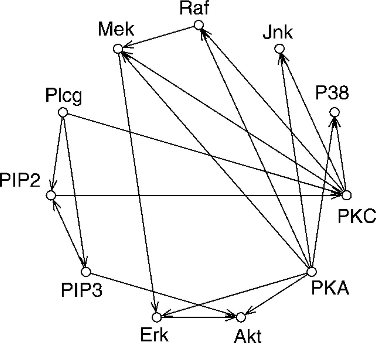
Figure 2: Original network derived in Sachs et al.
- \(p\) = 11 proteins
- \(n\) = 7466 cells
Cell signalling network
Same network, but from the original Sachs et al. paper: better biological interpretation.
Sachs et al. 2005
Cell signalling network
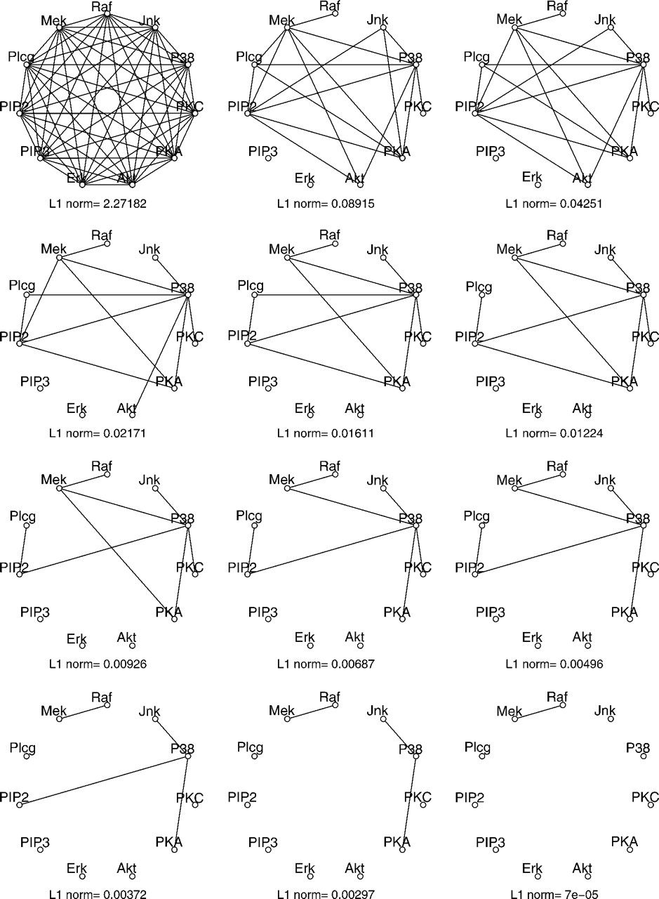
Figure 3: Undirected graphs generated using graphical lasso with various settings for
the regularization parameter, \(\rho\).
Cell signalling network
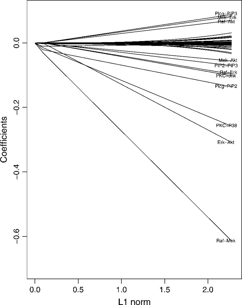
Figure 4: Profile of coefficients as the total \(L_1\) norm of the coefficient vector increases and \(\rho\) decreases. (The density of network increases as \(L_1\) increases.)
Cell signalling network
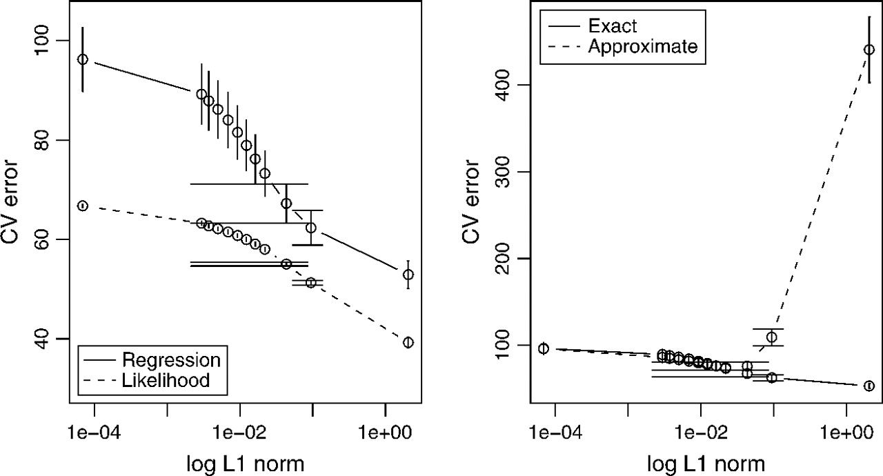
Figure 5: LHS - tenfold cross-validation. RHS - regression sum of squares of the exact graphical lasso vs. Meinhausen-Buhlmann approximation.
Summary
Summary
- Friedmann et al. present a fast \(L_1\) penalized approach for inducing sparsity in graphical models.
- Builds on previous methods, starting with the blockwise coordinate descent approach from Banerjee et al. (2007.)
- Method arrives at at exact result and performs significantly faster than previous methods.
- When tested on real data, however, model provides only an approximation and fails to predict many of the actual edge conditions.
- Free implementation of the graphical lasso written in fortran and R is
available:
glasso.
More info
For a more recent (Dec 2012) discussion on this problem, check out this Neural Information Processing (NIPS) talk by Po-Ling Loh:

No voodoo here! Learning discrete graphical models via inverse covariance estimation
References
- Nicole Baumgarth, Mario Roederer, (2000) A Practical Approach to Multicolor Flow Cytometry For Immunophenotyping. Journal of Immunological Methods 243 77-97 10.1016/S0022-1759(00)00229-5
- J. Friedman, T. Hastie, R. Tibshirani, (2007) Sparse Inverse Covariance Estimation With The Graphical Lasso. Biostatistics 9 432-441 10.1093/biostatistics/kxm045
- Nicolai Meinshausen, Peter Bühlmann, (2006) High-Dimensional Graphs And Variable Selection With The Lasso. The Annals of Statistics 34 1436-1462 10.1214/009053606000000281
- K. Sachs, (2005) Causal Protein-Signaling Networks Derived From Multiparameter Single-Cell Data. Science 308 523-529 10.1126/science.1105809
- Hastie Trevor, (2009) The elements of statistical learning data mining, inference, and prediction.
System info
sessionInfo()
## R version 3.0.2 (2013-09-25)
## Platform: x86_64-unknown-linux-gnu (64-bit)
##
## locale:
##  [1] LC_CTYPE=en_US.UTF-8       LC_NUMERIC=C
##  [3] LC_TIME=en_US.UTF-8        LC_COLLATE=en_US.UTF-8
##  [5] LC_MONETARY=en_US.UTF-8    LC_MESSAGES=en_US.UTF-8
##  [7] LC_PAPER=en_US.UTF-8       LC_NAME=C
##  [9] LC_ADDRESS=C               LC_TELEPHONE=C
## [11] LC_MEASUREMENT=en_US.UTF-8 LC_IDENTIFICATION=C
##
## attached base packages:
## [1] stats     graphics  grDevices utils     datasets  methods   base
##
## other attached packages:
## [1] knitcitations_0.4-7 bibtex_0.3-6        knitr_1.5
## [4] igraph_0.6.5-2      slidify_0.3.3       colorout_1.0-0
## [7] vimcom_0.9-9        setwidth_1.0-3
##
## loaded via a namespace (and not attached):
##  [1] digest_0.6.3   evaluate_0.5.1 formatR_0.9    httr_0.2
##  [5] markdown_0.6.3 RCurl_1.95-4.1 stringr_0.6.2  tools_3.0.2
##  [9] whisker_0.3-2  XML_3.98-1.1   xtable_1.7-1   yaml_2.1.8